Semantic Matching Without a Single Line of Training Data

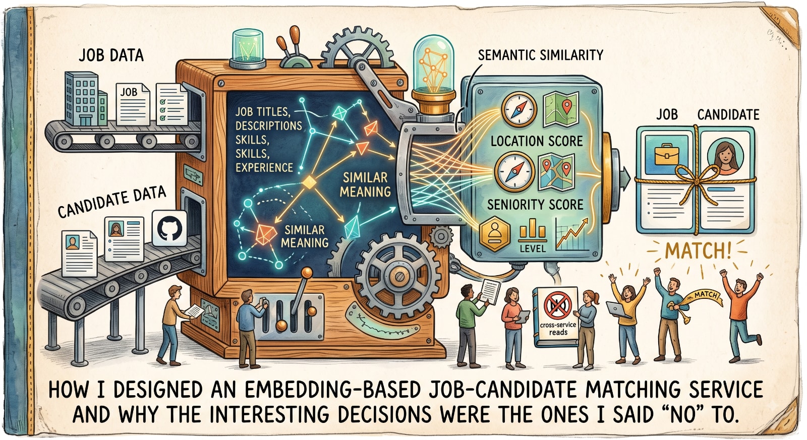
How I designed an embedding-based job–candidate matching service and why the interesting decisions were the ones I said "no" to.

---

The setup

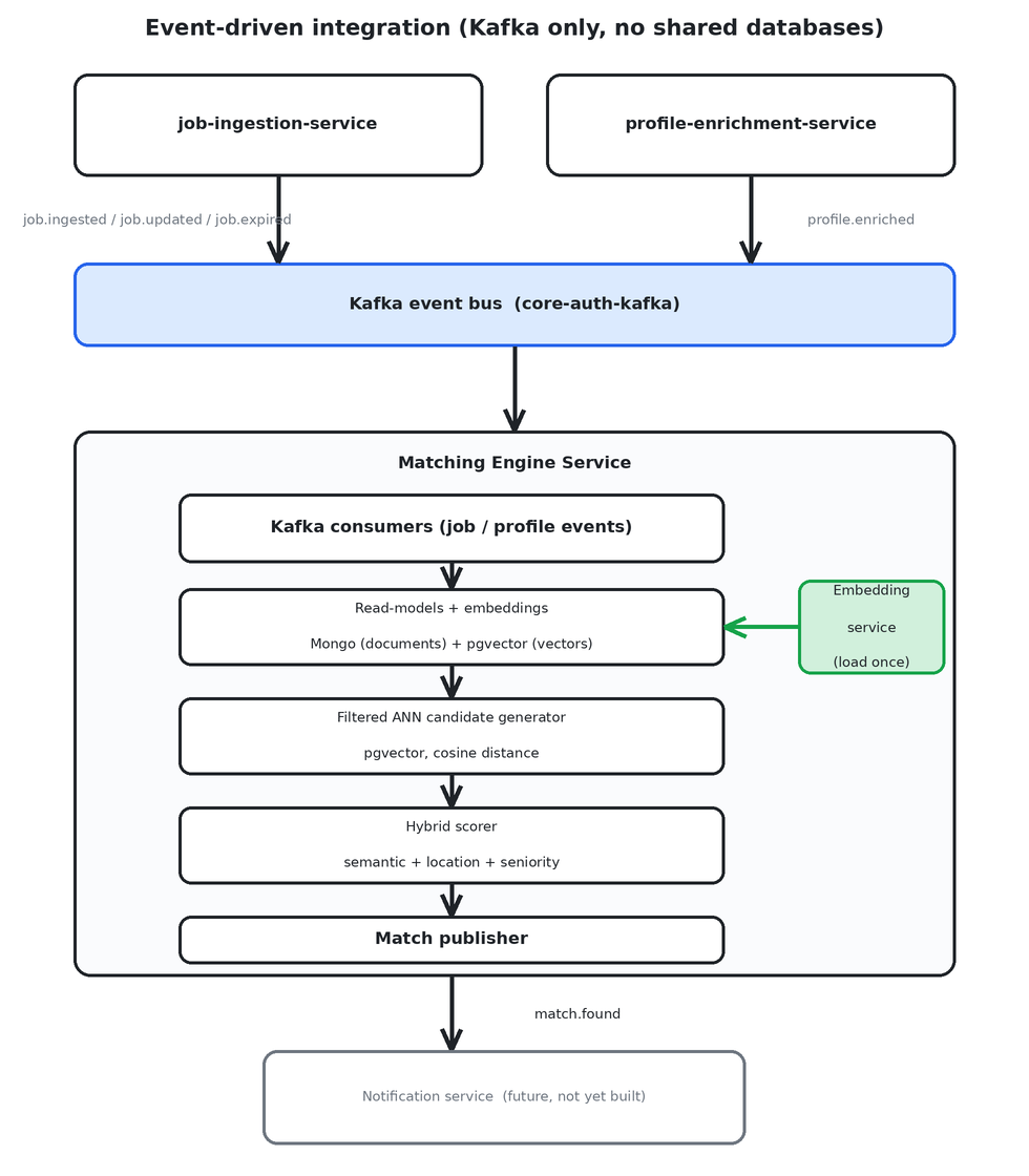
I'm building a job platform out of small, independent microservices. Two of them already work and produce real data:

• job-ingestion-service scrapes jobs and knows their title and description.
• profile-enrichment-service turns a user's resume and GitHub into structured skills, experience, and project summaries.

And between them: nothing. No service connected a job to a person. That's the gap the Matching Engine fills the thing that decides this job is a good fit for that candidate and says so.

The obvious question is how you decide "good fit." My first design answered it one way. My second design threw that answer out. This post is about why.

First instinct: count the overlapping skills

The original plan was rule-based: extract skills from the job, extract skills from the profile, score the overlap. It's simple, it's explainable, and — critically — it needs zero training data, which I don't have. Nobody has ever used the platform. There are no clicks, no applications, no "the user liked this match" signals to learn from. That's a cold-start problem, and it's real.

So rule-based skill overlap seemed like the disciplined choice. Then I actually looked at the data.

The jobs had no populated skills field. Just a title, and internally a description. The profiles had rich structured skills. So my "count the overlap" plan depended on both sides sharing a vocabulary of discrete tags — and one side had none. I'd have been comparing a full list against an empty one and papering over the gap with a neutral 0.5 fallback that meant nothing.

The plan wasn't wrong in spirit. It was wrong about the data.

The reframe: I conflated two different objections

Here's the mistake I'd made, and it's a common one. My reason for not using embeddings in v1 was "no training data, no users." But that reasoning quietly bundled two separate things:

1. Training a model — genuinely needs labeled outcome data I don't have. Still true. Still out of scope.
2. Using embeddings — does not need training data at all.

A pretrained sentence-embedding model is used at inference time. You hand it text, it hands back a vector, and semantically similar text produces nearby vectors — with zero examples from your domain. The model was already trained, by someone else, on a mountain of general text.

So the objection to "vector-based v1" (needing data I don't have) applied to a trained scoring model — which stays out of scope — but never to embeddings themselves. Once I separated those, the whole picture changed. Embeddings sidestep the empty-skills-field problem entirely: instead of requiring both sides to share discrete tags, they compare the meaning of whatever text exists. Job title + description on one side; skills + experience + projects on the other. No shared vocabulary required.

How embeddings turn "meaning" into geometry

An embedding is a fixed-length list of numbers — a point in high-dimensional space (384 dimensions, for the model I chose). The useful property: similar meaning → nearby points.

So "find good candidates for this job" becomes a geometry question: which profile points are closest to the job's point? The rest of this section is the math that makes "closest" precise. If you just want the architecture story, skip to the next section — but the math is genuinely the interesting part.

Measuring "close": three distances, and why cosine wins

Given two vectors $A = (a_1, \dots, a_D)$ and $B = (b_1, \dots, b_D)$, there are three standard ways to score how related they are.

Dot (inner) product — how much they point the same way, scaled by their lengths:

$$A \cdot B = \sum_{i=1}^{D} a_i b_i$$

Euclidean (L2) distance — straight-line gap between the two points:

$$d_{L2}(A,B) = \|A - B\| = \sqrt{\sum_{i=1}^{D} (a_i - b_i)^2}$$

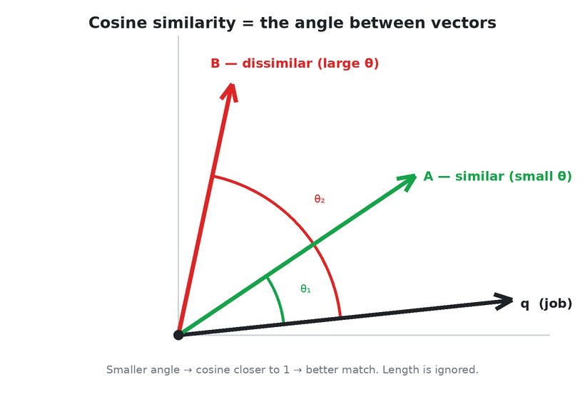
Cosine similarity — the angle between them, with length divided out:

$$\cos(\theta) = \frac{A \cdot B}{\|A\|\,\|B\|} = \frac{\sum_{i=1}^{D} a_i b_i}{\sqrt{\sum_{i=1}^{D} a_i^2}\;\sqrt{\sum_{i=1}^{D} b_i^2}}$$

Cosine runs from +1 (same direction) through 0 (perpendicular, unrelated) to −1 (opposite). I use cosine because direction carries the meaning, not magnitude: a long job description and a short one about the same role should match. Dividing by $\|A\|\|B\|$ throws the lengths away and compares pure orientation.

The three are secretly the same thing (when you normalize)

Here's the connective tissue that makes vector search efficient. If you L2-normalize each vector — rescale it to length 1, $\hat{A} = A / \|A\|$ — then two things collapse into one.

First, cosine similarity becomes the dot product, because the denominator is now 1:

$$\hat{A} \cdot \hat{B} = \frac{A \cdot B}{\|A\|\,\|B\|} = \cos(\theta)$$

Second, Euclidean distance becomes a monotonic function of cosine. Expand the squared distance:

$$\|\hat{A} - \hat{B}\|^2 = \|\hat{A}\|^2 + \|\hat{B}\|^2 - 2\,\hat{A}\cdot\hat{B} = 1 + 1 - 2\cos(\theta) = 2\bigl(1 - \cos\theta\bigr)$$

So $\|\hat{A} - \hat{B}\| = \sqrt{2(1 - \cos\theta)}$. As cosine goes up, Euclidean distance goes down — always, no exceptions. That's why an index that only knows how to sort by Euclidean distance can still answer cosine-similarity queries perfectly, as long as the vectors are normalized. Ranking by one is identical to ranking by the other. Many embedding models (including the one I use) output normalized vectors precisely so this shortcut holds.

A fully worked example (3 dimensions, so you can check it by hand)

Take a job vector and two candidate profiles:

$$q = (2,\,1,\,0), \qquad A = (1,\,1,\,0), \qquad B = (0,\,1,\,2)$$

Profile A:

$$q \cdot A = (2)(1) + (1)(1) + (0)(0) = 3$$ $$\|q\| = \sqrt{4 + 1 + 0} = \sqrt5 \approx 2.236, \qquad \|A\| = \sqrt{1 + 1 + 0} = \sqrt2 \approx 1.414$$ $$\cos(q, A) = \frac{3}{2.236 \times 1.414} = \frac{3}{3.162} \approx 0.949 \;\Rightarrow\; \theta \approx 18.4°$$

Profile B:

$$q \cdot B = (2)(0) + (1)(1) + (0)(2) = 1, \qquad \|B\| = \sqrt{0 + 1 + 4} = \sqrt5 \approx 2.236$$ $$\cos(q, B) = \frac{1}{2.236 \times 2.236} = \frac{1}{5} = 0.200 \;\Rightarrow\; \theta \approx 78.5°$$

So A (18°) is a strong match and B (78°) is nearly unrelated — which matches intuition: $A$ leans the same way as $q$, $B$ points off into a different axis. Two dot products and a couple of square roots, and you've ranked your candidates.

From distance back to a score

pgvector doesn't hand you similarity directly — it exposes a cosine distance operator, <=>, defined as

$$d_{\cos} = 1 - \cos(\theta)$$

which runs 0 (identical direction) → 1 (perpendicular) → 2 (opposite), since cosine spans $[-1, +1]$. For my two profiles: $d_{\cos}(q,A) = 1 - 0.949 = 0.051$ and $d_{\cos}(q,B) = 1 - 0.200 = 0.800$.

I want a similarity in $[0, 1]$ to feed the final score, so I convert:

$$\text{sim} = 1 - \frac{d_{\cos}}{2}$$

Substituting $d_{\cos} = 1 - \cos\theta$ shows exactly what this does:

$$\text{sim} = 1 - \frac{1 - \cos\theta}{2} = \frac{1 + \cos\theta}{2}$$

It's an affine remap of cosine's $[-1, +1]$ onto $[0, 1]$: identical → 1, perpendicular → 0.5, opposite → 0. For A: $\text{sim} = 1 - 0.051/2 \approx 0.974$. For B: $\text{sim} = 1 - 0.800/2 = 0.600$. (This is the one-liner in my scorer, and the reason its unit test asserts $0 \to 1$, $1 \to 0.5$, $2 \to 0$.)

A note on high dimensions

You might worry: in 384 dimensions, doesn't the "curse of dimensionality" make distances meaningless? In uniformly random high-dimensional data, yes — pairwise distances concentrate and everything looks equidistant. Embeddings dodge this because they don't fill the space uniformly; a good model places related concepts on a much lower-dimensional manifold curled up inside those 384 dimensions. The ambient dimension is 384, but the effective structure the model learned is far smaller, and that's where cosine stays discriminative.

The decision I'm proudest of: refusing the shortcut

Embeddings need text to embed. On the profile side, I had plenty. On the job side, the rich text — the description — lived in job-ingestion-service's database but was not published in its events. The events were deliberately slim envelopes: just a title.

There was a tempting shortcut: have the Matching Engine reach into job-ingestion's database and read the description directly. One query. Done.

I didn't, and I want to explain why, because this is where architecture actually earns its keep.

The whole platform runs on one rule: every service owns its data, and services talk only through events. Nobody reads anybody else's database. The moment the Matching Engine queries job-ingestion's Mongo, those two services are welded together — you can't change one's schema, deploy it, or scale it without minding the other. The independence that made microservices worth the trouble is gone.

So instead of a shortcut, the missing text became a real, scoped piece of work: extend job-ingestion's event schema to include description_text, version-bumped and tested like any other change. It's more work. It's the right amount of work.

And until that ships, the Matching Engine doesn't pretend. It embeds jobs on the title alone, labels each one title_only, logs it as degraded, and tracks the percentage of properly-embedded records as a first-class metric. The system keeps working, just less well — and I can see that it's degraded instead of being silently lied to. Degraded-but-visible beats broken-but-hidden.

Storing and searching the vectors: the boring choice was correct

Once you have thousands of vectors, you need to search them fast. The industry-default answer is a dedicated vector database like Pinecone — a separate managed service with its own account, API key, and monthly bill.

I already run a PostgreSQL instance. Postgres has an extension, pgvector, that stores vectors and does similarity search inside the database I already operate. At my scale — thousands of records, not billions — pgvector is more than enough. Choosing Pinecone would have meant a new service to run, back up, monitor, and pay for, solving a scaling problem I don't have.

For a platform run by one person, "one fewer thing to operate" is a feature. The simplest tool that solves the actual current problem won.

A word on ANN — the "approximate" is a feature

Searching vectors exactly means comparing your query to every stored vector. With $N$ vectors of dimension $D$, that's

$$O(N \cdot D)$$

work per query — a distance computation is $D$ multiply-adds, done $N$ times. At $N$ in the thousands and $D = 384$ that's a few million operations: instant. At $N$ in the hundreds of millions it's a non-starter for every single query. Approximate Nearest Neighbor (ANN) search trades a sliver of accuracy for a huge speed win — it might occasionally return the 2nd-closest match instead of the 1st, which for job matching is completely harmless.

Two families of index make this trade, and pgvector supports both:

IVFFlat partitions the vectors into $L$ clusters (via k-means) with a centroid each. A query compares itself to the $L$ centroids, picks the nearest $p$ clusters (probes), and only brute-forces inside those. Cost drops from $N$ to roughly

$$O\!\left(L \cdot D \;+\; \frac{N}{L}\cdot p \cdot D\right)$$

— the first term finds the right clusters, the second searches them. It's approximate because the true nearest neighbor can sit just across a cluster boundary you didn't probe; raising $p$ buys accuracy back at linear cost.

HNSW (Hierarchical Navigable Small World) — my default — builds a multi-layer graph. Every vector is a node linked to its $M$ nearest neighbors; higher layers keep only a thinning subset with long-range "express-lane" links, the bottom layer holds everything densely. A search enters at the top, greedily hops to whichever neighbor is closest to the query, descends a layer, repeats — coarse long jumps up top, fine refinement at the bottom. Because each layer roughly halves the remaining distance, search touches on the order of

$$O(\log N)$$

nodes instead of all $N$ — binary-search-through-space. Building the graph costs about $O(N \log N \cdot M)$ once, up front. The knobs: $M$ and ef_construction control graph quality at build time; ef_search sets how wide a candidate list the query keeps — larger means closer to exact, at more work. HNSW is approximate because a purely greedy walk can settle into a local best and miss the global one; a bigger ef_search makes that rare.

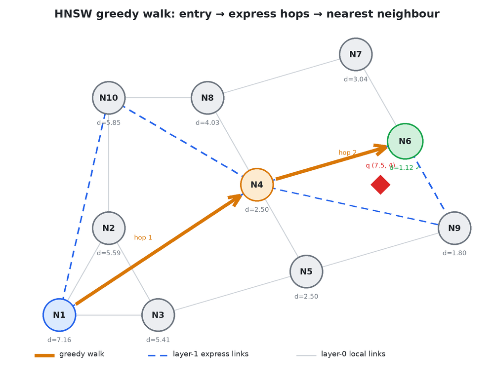
The headline: exact search scales like $N$, HNSW like $\log N$. That gap is the entire reason ANN exists.

Keeping the score honest

The last decision: even with embeddings, I refused to publish a single opaque number. Semantic similarity is one signal, but it can't tell you a remote-only candidate is being matched to an on-site job, or that a junior is being matched to a staff role. So the published score is a weighted sum of three interpretable components:

$$\text{score} = w_{\text{sem}}\cdot s_{\text{sem}} \;+\; w_{\text{loc}}\cdot s_{\text{loc}} \;+\; w_{\text{sen}}\cdot s_{\text{sen}}$$

with each sub-score $s \in [0,1]$ and the weights summing to 1 ($w_{\text{sem}}=0.6,\; w_{\text{loc}}=0.25,\; w_{\text{sen}}=0.15$), which guarantees the total also lands in $[0,1]$. Concretely, take Profile A from the earlier example — semantic similarity $s_{\text{sem}} = 0.974$ — and say it's a remote job ($s_{\text{loc}} = 1.0$) with a one-level seniority gap ($s_{\text{sen}} = 0.75$):

$$\text{score} = 0.6(0.974) + 0.25(1.0) + 0.15(0.75) = 0.584 + 0.25 + 0.113 = 0.947$$

A strong match — and I can see why: high on all three axes. The weights are configuration, not code, so I can re-tune the balance without a deploy.

Each sub-score has an honest rule behind it. Location is a soft signal — a remote job scores 1.0 for everyone, otherwise it's the overlap of location tokens, and an unknown location is a neutral 0.5 rather than a zero. Seniority decays with the ordinal gap between levels: same level scores 1.0, and I subtract 0.25 per step of distance, $s_{\text{sen}} = \max(0,\; 1 - 0.25\lvert \ell_{\text{job}} - \ell_{\text{profile}} \rvert)$, so a senior-vs-mid gap of one level gives 0.75.

The semantic part is admittedly a black box — you can't decompose "why are these two vectors close." But location and seniority stay fully checkable. So when a match looks weird, I can still recompute two of the three components by hand. With no real users to validate against, that partial explainability is my only ground truth.

What I deliberately did not build

The discipline of a design is as much in the cuts as the features. Explicitly out of scope, and staying there:

• No trained or fine-tuned model — still a cold-start problem; revisit only when real usage data exists.
• No dedicated vector DB — pgvector until scale actually forces the question.
• No cross-service database reads — the rule that made the schema-extension work necessary.
• No fully opaque scoring — always a breakdown.

Each of these was a decision, not a default. Writing them down means the next person (probably future me) knows they were chosen, not forgotten.

Does this actually scale?

The reasonable objection to all of this is: "sure, it's elegant at a thousand records — what happens at a million?" It's worth being precise, because the intuitive answer (bigger catalog → slower matching) turns out to be mostly wrong.

The cost is per-event, not per-record. This is the property that everything hinges on. When a job arrives, I don't compare it to every candidate — one ANN query returns the top $N$ ($N = 50$), I score those 50, and I'm done. So the work to process a single event is roughly

$$\underbrace{O(1)}_{\text{embed}} \;+\; \underbrace{O(\log P)}_{\text{ANN over } P \text{ profiles}} \;+\; \underbrace{O(N)}_{\text{score top-}N}$$

The middle term grows only logarithmically with catalog size $P$; the last term is a constant no matter how large the catalog gets. Doubling the number of users does not double the work to match one job. That's the entire reason I designed the N×M cross-product out and never let a "compare everything to everything" query exist. The thing that scales linearly is event throughput — how many jobs and profiles change per second — not how many exist.

Storage is the least of it. Each embedding is 384 floats × 4 bytes ≈ 1.5 KB. Twenty thousand records is ~30 MB; two million is ~3 GB of vectors plus roughly double that for the HNSW index in RAM. Postgres is comfortable there. It's around the low tens of millions of vectors that the index stops fitting nicely in memory — and that, precisely, is the "measured bottleneck" I keep promising to revisit rather than pre-solve.

What actually breaks first — and it isn't the vectors:

1. Kafka consumer throughput. A single consumer loop only processes so many events per second. The fix is boring and horizontal: partition the topics by id and run a consumer group. This is exactly why I insisted on idempotency and per-key ordering — a consumer rebalance re-delivers events, and full-replace writes plus publish-only-on-transition make that replay harmless. Config and deploy, not a rewrite.
2. Re-evaluation fan-out — the real trap. The danger was never a new job; it's the temptation to "re-match everything" when weights change, which is the O(J × P) explosion the whole design exists to avoid. The discipline is to keep evaluation strictly incremental: one event, one top-N query. Never build the batch job that quietly reintroduces the cross-product.
3. The candidate pre-filter. I ship the location/seniority-filtered id list into the vector query. Fine when the filter matches a few hundred profiles; a problem when it matches a hundred thousand. The escalation is known and written down — move the filter fields alongside the vectors so the index filters natively in one query, instead of passing a giant id list around.

Notice what's not on that list: a rewrite, a new database, a change to the service boundaries. Every lever above is operational — partition a topic, keep a query incremental, move a filter column. The dedicated vector database only earns its keep at the far end (tens of millions of vectors), and until then paying for it would be solving a problem I don't have — the same discipline that picked pgvector in the first place.

The honest caveat: none of this is measured. The scaling shape is sound by construction, but the service hasn't run under load, so I don't actually know where the knee is. The first real scaling task isn't optimization — it's measurement: load the pgvector query and the consumer with a hundred thousand synthetic records and find out where reality diverges from the back-of-envelope. Estimating the bottleneck is not the same as having found it.

The takeaway

The best decisions in this design weren't clever. They were about matching the tool to the actual problem and refusing the shortcuts that trade long-term independence for short-term speed:

• Separate "can't train a model" from "can't use embeddings" — they're different problems.
• Solve a missing-data gap with a real schema change, not a database backdoor.
• Pick the boring tool (pgvector) that you already run.
• When you must degrade, degrade visibly.
• Keep the score explainable enough to sanity-check when you have no users to check against.

None of that requires training data. All of it requires being honest about what you actually have.

---

The Matching Engine is event-driven and connects to the rest of the platform purely through Kafka topics — it consumes job and profile events, publishes match.found, and knows nothing about who's listening. That decoupling is a story for another post.